

Most fleet decisions on crop farms get made backwards. Somebody looks at last season's breakdown, the frustration of waiting three days for a rental combine, and buys another machine "so this never happens again." Then that machine sits in the shed 340 days a year, depreciating, while the loan payment eats into a season where corn barely cleared breakeven.
The problem isn't that farmers can't do math. It's that fleet sizing is a peak‑window problem, not an annual‑average problem, and those two framings lead to completely different answers. Your fleet has to clear a specific number of acres inside a weather‑constrained window — everything outside that window is basically noise for this decision.
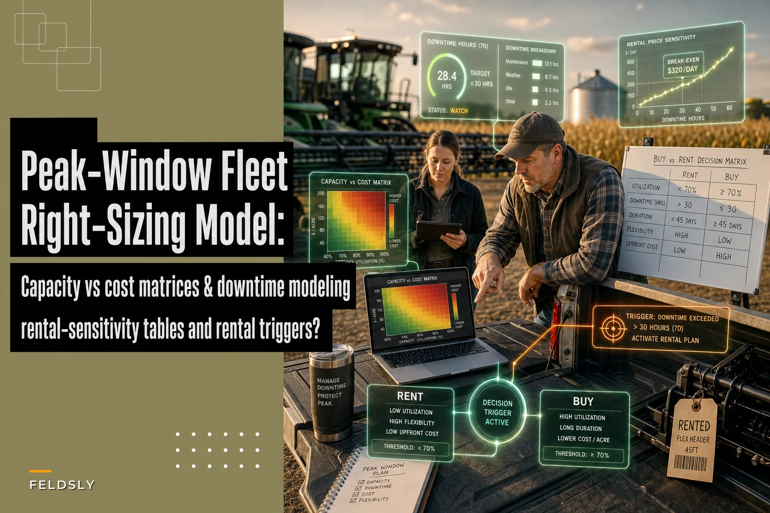
This piece walks through a right‑sizing model built around that window: a capital‑vs‑rental decision matrix, downtime modeling so you plan around breakdowns instead of pretending they won't happen, and sensitivity tables for when rental prices spike exactly when you need the machine. A solid farm fleet right sizing model is one you can stress‑test against a bad year, not just an average one.
Start with the window, not the fleet
The single most useful number in this exercise is your effective field capacity during the peak window — and how many working hours that window actually contains.
Most people go wrong at the same point. They'll say "we have a 12‑day planting window." But that's a calendar window. Inside it, you lose days to rain, half‑days to fields too wet to travel, hours to fog and dew burn‑off, and time to refills, moves between fields, and the inevitable clogged row unit. What looks like 12 days is often 6 to 7 genuinely productive ones.
A worked version for a corn operation:
-
Calendar window
12 days
-
Historical rainout/too‑wet loss
~30% → 8.4 usable days
-
Daily productive field hours (dew, fog, breakdowns, moves)
~10.5 of a 14‑hour day
-
Effective productive hours in window
~88 hours
Now the capacity question gets real. If you're farming 2,400 acres of corn that all needs to go in that window, you're looking at roughly 27 acres per productive hour. A 24‑row planter running 5.5 mph on 30" rows does maybe 22–26 acres/hour before you account for point rows and refills. One planter is right at the edge — one bad weather year and you're planting into June.
That "right at the edge" feeling is exactly where the capital‑vs‑rental decision lives.
The capital vs rental decision matrix
Once you know the window and the acres, every machine falls into one of four buckets. The mistake is treating all of them as "buy" decisions.
Take control of your farm’s productivity.
Feldsly helps you plan, track, and optimize every farming operation with precision.
- Centralized crop scheduling
- Resource & labor management
- Real-time weather alerts
No credit card required
| Utilization pattern | Peak‑window criticality | Best ownership call | Why |
|---|---|---|---|
| High hours, spread across season | High | Own | Amortizes well, always need it, control matters |
| Low annual hours, but critical in one window | High | Own primary, rent surge | Owning full backup is dead capital |
| Low hours, low criticality | Low | Rent or custom hire | No reason to tie up capital |
| High hours but timing flexible | Medium | Own, size conservatively | You can shift work in time |
The second row is where most of the money hides. Think about a grain cart, a second planter, or a supplemental combine. You don't need two combines for 300 hours a year — you need a second combine for maybe 40 hours during a moisture‑sensitive stretch. That's a rental or custom‑harvest conversation, not a $450k purchase.
A pattern worth naming: farms consistently over‑own primary iron and under‑plan surge capacity. They buy the second combine and then still get caught because both machines went down the same wet week, or because the surge they actually needed was grain cart and truck capacity, not more heads in the field.
The cleaner framing: own what you use across the whole season and can't afford to wait on. Rent or contract the stuff whose entire value is compressed into a handful of window hours.
Downtime modeling — plan the breakdown into the schedule
Any capacity plan that assumes 100% uptime is fiction. The useful move is baking expected downtime into the window math so your plan survives contact with a real season.
-
Rough failure likelihood in‑window — from your own history. If your combine has thrown a meaningful failure in 3 of the last 5 harvests, that's a 60% chance you lose some time.
-
Typical downtime hours per event — parts run, dealer wait, field repair. Be honest; "a couple hours" is usually a full day once you count the drive to the dealer.
-
What that downtime costs in the window — acres you can't cover × the value of getting them in on time (yield loss, moisture premium lost, quality downgrade).
Back to that single‑planter corn operation. Suppose there's a 40% chance of a downtime event costing around 10 productive hours. Ten hours at 24 acres/hour is 240 acres pushed out of the ideal window. If pushing those acres late costs roughly $18–$25/acre in yield drag, that's a $4,300–$6,000 expected‑value hit before you even start talking about a full‑season delay cascade.
Suddenly a $9,000 rental trigger for a backup planter during that specific week doesn't look expensive. It looks like insurance priced right at the actuarial line.
This is also why a real machinery lifecycle plan pays for itself — a lot of "surprise" downtime is predictable wear that a governance schedule catches. We covered that side of things in the peak‑season breakdown prevention playbook; treat it as the upstream control that lowers the failure probabilities feeding this model.
A simple downtime workflow
-
Log every in‑window downtime event with cause, hours lost, and acres affected — one line, phone‑captured.
-
At season end, roll it into per‑machine failure rates.
-
Feed those rates back into next year's window math as expected lost hours.
-
Set a rental trigger threshold
"if we lose more than X hours by day 3 of the window, the backup call goes out."
A simple visual of that loop:
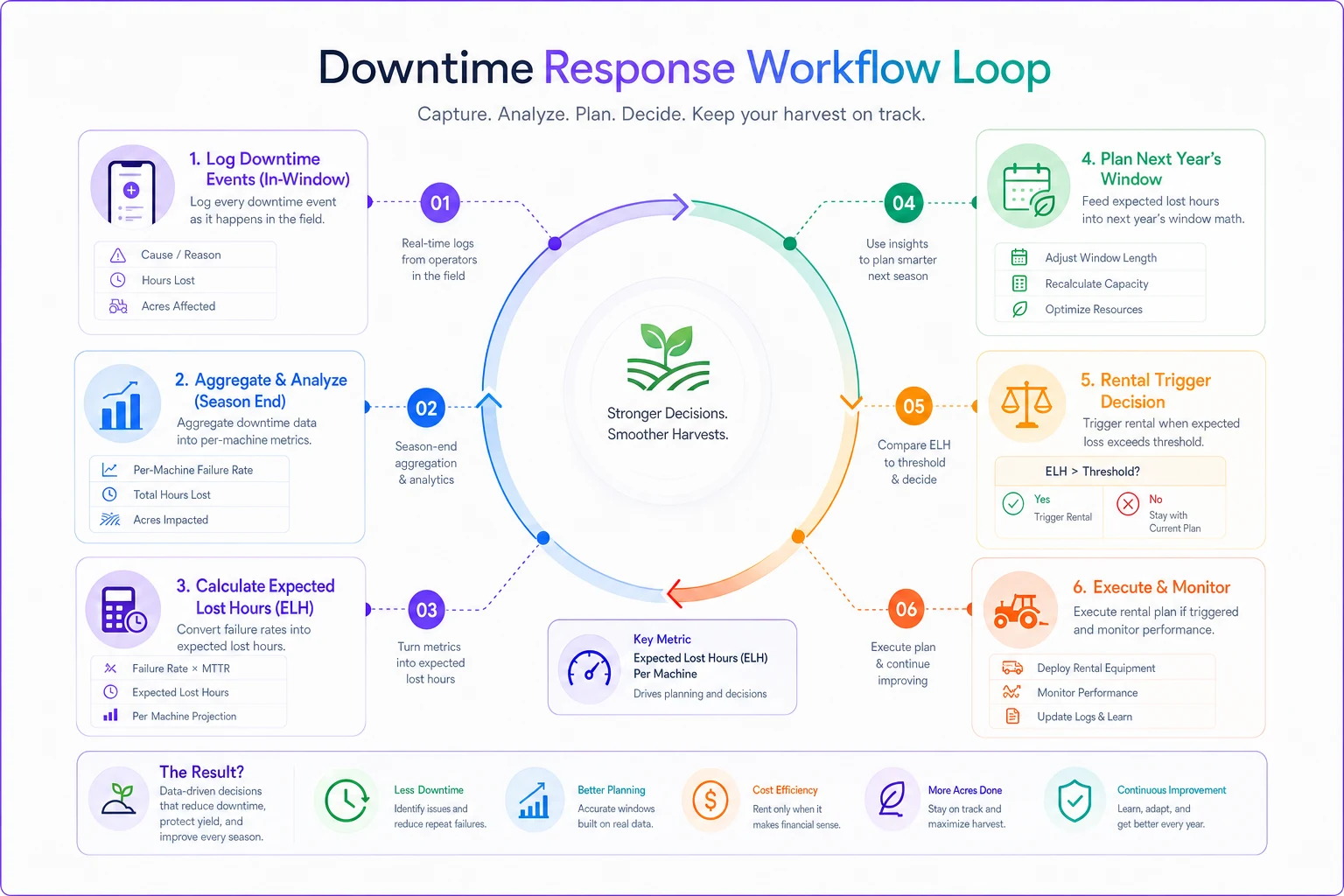
The trigger matters more than the model. A plan that says "we'll rent if things go bad" without a number attached always rents too late, because everyone hopes the machine comes back tomorrow.
Having that trigger documented somewhere accessible — not just in one person's head — is where a lot of operations fall down. When the breakdown happens at 7pm on day two of the window, someone needs to be able to pull up the threshold and make the call without a committee meeting.
Rental‑price sensitivity — the part everyone gets wrong
You build a clean model, decide renting surge capacity is cheaper than owning, and pencil in $3,500 for a week‑long combine rental. Then a derecho or an early frost hits your whole region at once, every farm within 200 miles wants the same machine, and that $3,500 rental is now $6,000 — if you can even get it.
Rental economics are correlated with exactly the conditions that make you need the rental. That correlation is probably the most under‑modeled risk in fleet planning.
So you stress‑test it. Build a sensitivity table showing how your "rent vs own" answer shifts as rental prices spike and availability tightens.
| Rental price scenario | Weekly rental cost | Times you'd rent per 5 yrs | 5‑yr rental cost | Vs. owning (annualized ~$38k) |
|---|---|---|---|---|
| Normal market | $3,500 | 3 | $10,500 | Renting wins big |
| +40% peak spike | $4,900 | 3 | $14,700 | Renting still wins |
| +75% regional shortage | $6,100 | 4 (need it more in bad years) | $24,400 | Renting wins, narrowing |
| Spike + can't source (custom hire premium) | $8,500 effective | 4 | $34,000 | Roughly a wash |
Two things jump out. First, renting has to get very bad before owning wins — ownership carries cost every single year whether you need it or not. Second, the real risk isn't price, it's availability. The bottom row isn't about $8,500; it's about the year you needed the machine, everyone else did too, and you couldn't get one at any price.
That changes the strategy. Instead of "own vs rent," the smart position is often rent, but lock the option. A pre‑season standby agreement or a first‑call arrangement with a dealer or custom operator — sometimes for a modest reservation fee — buys you availability certainty for a fraction of ownership cost. You're paying to not be the farm calling at 6am on the first dry day of a regional shortage.
Seasonal capacity checklist
Run this before each major window — planting and harvest separately, because the constraints differ.
-
- [ ] Recalculate effective productive hours for this window using the last 3–5 years of weather loss, not the calendar count.
-
- [ ] Confirm peak acres that genuinely must move in this window vs. acres with timing flexibility.
-
- [ ] Divide it out
acres per productive hour required vs. your fleet's real field capacity (derated for point rows, refills, moves).
-
- [ ] Flag any machine "at the edge" — if one machine covers 90%+ of required capacity with no slack, that's your rental/backup candidate.
-
- [ ] Pull per‑machine downtime history and set expected lost hours for each critical unit.
-
- [ ] Set explicit rental triggers — the number of lost hours or the calendar day that fires the backup call.
-
- [ ] Confirm surge availability now, not during the window — call the dealer/custom operator, get standby terms in writing.
-
- [ ] Stress‑test rental cost at +40% and +75% and check whether your decision flips.
-
- [ ] Line up the support fleet — grain carts, trucks, tender trailers. Combine capacity is useless if trucks are the bottleneck.
-
- [ ] Match crew to iron — a rented machine with nobody trained to run it isn't capacity.
The line item people skip most is the second‑to‑last one. A farm will obsess over combine hours and then bottleneck the whole harvest on truck cycle time to the elevator. Right‑sizing the fleet means right‑sizing the whole chain, not just the machine in the field.
A real scenario
A roughly 3,100‑acre corn and soybean operation in the eastern Corn Belt ran two owned combines for years, one of them an older backup that mostly existed "just in case." That backup tied up around $32k of capital plus insurance and shed space, and ran maybe 45 hours a season.
They ran the window math and found their newer combine alone cleared the harvest window in a normal year with a couple days of slack. The old machine wasn't buying capacity — it was buying comfort. And its uptime was so poor that in the two years it was needed, it broke down anyway.
They sold it, freed up the capital, and set up a first‑call custom‑harvest arrangement plus a standby rental agreement with a modest pre‑season fee. Over the next three seasons they triggered outside help twice. Their all‑in cost for surge capacity ran somewhere in the $7k–$9k range across those years — against the $32k of dead capital plus carrying costs they'd been sitting on.
The part that mattered most wasn't the money. Both times they called, the machine actually showed up and ran, because the availability was arranged in August, not begged for in October. The old backup had failed them precisely when they needed it; the arranged surge didn't.
When this model makes sense — and when it doesn't
This makes sense when:
-
Your acreage is concentrated in tight, weather‑constrained windows.
-
You have machines that are "just in case" and rarely run.
-
There's a functioning rental or custom market in your area.
-
You can capture downtime and weather‑loss history to feed the math.
This is a bad idea when:
-
You're in a region with genuinely no rental or custom availability — then owning surge capacity is the only real option and the model just tells you how much.
-
Your windows are wide and your acreage modest enough that you're never near capacity — you likely already have slack and don't need to optimize.
-
You can't or won't track downtime honestly, in which case the sensitivity tables are built on guesses.
Who should skip this entirely: very small operations where a single reliable machine clears everything with room to spare. Modeling surge capacity you'll never use is its own form of over‑engineering.
Tie the fleet plan to the money plan
Fleet right‑sizing decisions don't live alone — they're a big line in your commodity‑year budget, and the "own vs rent" call should flex with the price scenario you're planning around. In a tight‑margin year, freeing $30k+ of capital and shifting to arranged surge capacity can be the difference between a planting plan that pencils and one that doesn't.
That connection is worth building deliberately. The fleet decision and the budget scenario belong in the same conversation, not separate spreadsheets reviewed at different times of year. It fits directly into the tiered budgeting approach we laid out for operational financial scenario planning.
The goal here isn't to own less iron for its own sake. It's to stop letting a bad memory from one wet week drive a six‑figure capital decision. Size the fleet to clear the window, plan the breakdowns into the schedule instead of hoping against them, and stress‑test your rental assumptions against the exact conditions that make rentals scarce. Do that, and you'll spend your capital where it actually protects yield — and keep the rest working somewhere more useful than the back of the shed.
Ready to revolutionize your farm management?
Join 500+ farms using Feldsly to boost yields, reduce waste, and streamline daily farm workflows.